Everyone here at Clicks and Clients can tell you I’m somewhat of an Excel snob. I love excel, it can accomplish very complex tasks in a very short amount of time once you’ve become familiar with the some of the wonderful features and formulas it has. One of our common question we ask for new hire interviews is “On a scale of 1-10, how would you rate your experience with excel”. The overwhelming majority of people rate themselves at a 6 or a 7. Let’s evaluate what a 1-10 scale of Excel experience might look like if we rate individual experience with  the tabs in the ribbon. 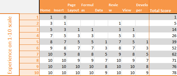When you look at Excel from the ribbon, many people realize just how much Excel can do that they didn’t even realize. Most people who rank themselves at a 6 or 7 have never worked in the Developer tab and most likely only have very surface level formula experience. I think for most people it’s a matter of ignorance, they aren’t aware of the things Excel can do but they have been successful with the simple tasks they have used Excel for in the past so they rate themselves highly.

8 Excel Tips this SEO can’t live without

#1 Remove duplicates

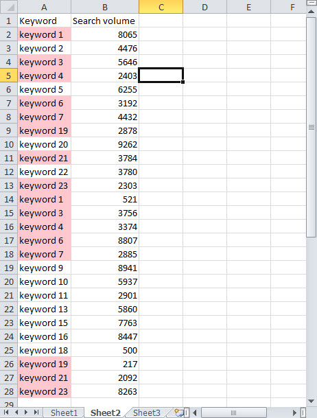
Remove duplicates is one of the easiest and most common features I use in Excel. In SEO, it’s a great way to clean up data. For example, when I perform keyword research, I often find I’ll use multiple tools to collect the keywords then I paste the keyword data into a spreadsheet. So my spreadsheets start to look like this:

To remove the duplicate values, I select the top left of my table, or A1 then click on ‘Remove Duplicates’ from the Data ribbon.

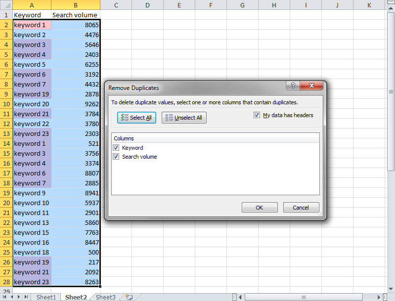
Notice that Excel selected my data range for me, make sure it’s done this properly, and make note if the headers in the data are selected. In this screenshot, Excel selected the headers so I want to indicate that my data does have headers in the dialog box. If I only want to remove the rows where my keyword is duplicated, I can simply select only that column.

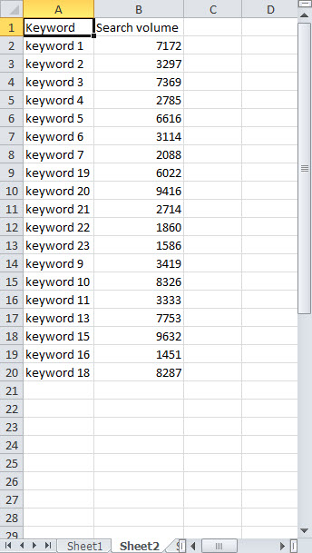
When it’s done it will have removed the rows in my data with duplicate values, ensuring that my search volume data is moved to stay next to it’s keyword.

#2 Tables

Tables make several elements of Excel more easily accessible and they look nice so I find I use them a lot to make working with large data sets easier. My most common use of these in with Screaming Frog SEO Spider data exports. 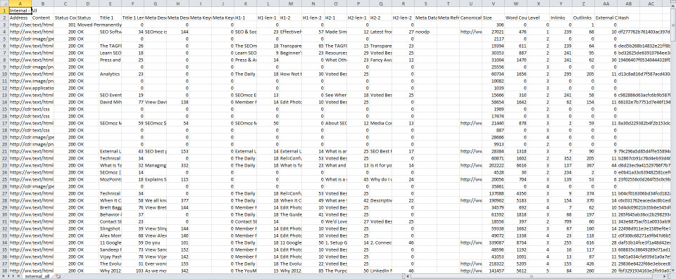Obviously this table has a lot of data, but it can be annoying to sort or filter data without tables. So I delete the first row then select the top left of the table, or A2 and click on ‘Table’ in the Insert ribbon. 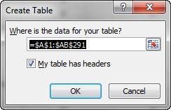In this case, I ensure that My table has headers is selected and click ok. Now that I have tables, I can sort or filter on any of the columns in my table. It also makes formulas easier to work with since Excel will automatically apply a formula to all rows in the table. If for example I wanted to create a formula to show just the directory of the page I could insert a column in front of column B.

Maybe I also want to see just those pages that had a 301 response. So I select the down arrow in the status code cell to open the filter and sort options for that column: 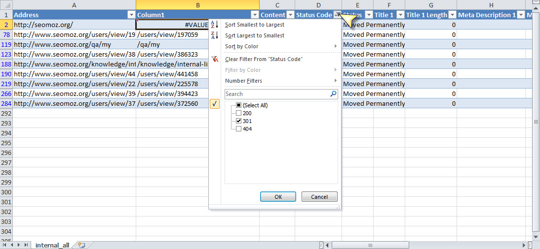As you can see, I simply select the values I want to appear in my data then select OK and Excel hides the rows of data that don’t meet those values.

#3 Excellent Analytics

Excellent Analytics uses the Google Analytics API to remotely collect your analytics data into Excel. Most people view most of their data directly in analytics but what about collecting that data into Excel so you can provide custom reports to your clients? How do you efficiently export the important bits of data you need each week or each month without needing to manage the CSV’s and copy and paste the data regularly into a format that works for your reporting?

Excellent Analytics makes this process much easier, but it’s not entirely perfect. Once you have it installed, it will appear as a new tab in the ribbon at the top of Excel.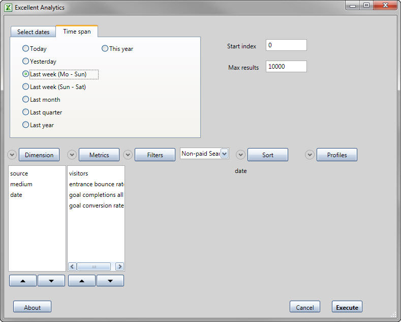

And here’s the data that is fed back:

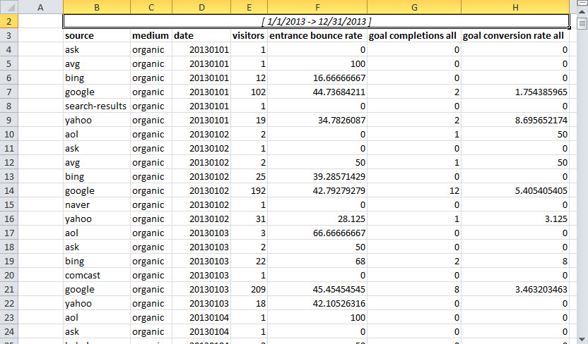As you see, you get a lot of data back, and though it can take some parsing it’s extremely easy to collect huge amounts of data. 20 domains with an entire year of Excel data can be output in 30 seconds, a task that could take an hour or more from Excel exports from analytics. The other issue is that you can consolidate data fairly well, often avoiding the need to do multiple exports from analytics since you’re able to display exactly what you want from one query with Excellent Analytics.

#4 Manual Calculation Controls

As you start to develop reporting or advanced use formulas in Excel you may find that your computer isn’t able to calculate the changes you make in Excel as fast as you’d like. You insert a column or row then the whole spreadsheet goes through and recalculates all cell formulas. This calculation may take only a second or it may take several minutes if you’ve gotten really adventurous in your formula use. Here’s how to configure Excel calculations to make life easy:

1. Select File
2. Options
3. Formulas
4. Select the Manual option under Wookbook Calculation

From now on, in order for the calculations to occur you’ll need to press F9 to calculate the whole spreadsheet or Shift+F9 for just your current worksheet. After a little time this becomes muscle memory and you will never want automatic calculation to be enabled again.

#5 External file references

For regular reporting needs with careful consideration for large data sets and long term stability, external file references are undoubtedly the most important Excel function in my opinion. The easiest way to use indirect file references is to simply be working out of 2 spreadsheets, then to click from one to the other in an appropriate formula. The easiest example would be a direct cell reference like this:

Excel will create this same formula if you select a cell  type “=” in the formula box, then select a cell in another open spreadsheet. Obviously, the result will just be the value that is contained in the cell reference but this can be used in any formula such as a vlookup or index. As an example, lets pretend we have all our analytics data in separate xlsx files we save monthly but we have a reporting spreadsheet we use to collect data from analytics and build graphs and provide a dashboard overview of the analytics data. Being able to create the dashboard in one spreadsheet and store the analytics data separately makes file size management easier and it’s also better in the long run for fast calculations. The best part about external file references  is that you don’t need to necessarily have all external files open to be able to read data from them. Make your spreadsheets and reports talk, you’ll find you can start to generate more powerful and easier reports in less time!

#6 Indirect formula usage

As you start to realize the potential for external file references, you’re likely to encounter a issue that makes their use limited. For example, if you’re saving your files on a monthly basis, is there a way to make the external file reference understand that you want it to pull from a specific monthly file? The best way to describe this issue is to show you an example:

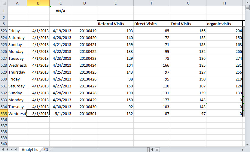
If you’re dragging a formula in columns E through H, how do you tell row 535 to pull from a different file from the rows above it? Since you’re collecting the data from a monthly analytics spreadsheet, you might use a month based file name. This is where indirect can be invaluable. To start with, there are a couple syntax rules that you need to know to read the formula correctly. Any time we want to put the text of what we want to use as a cell reference we inclose it in quotes “““. So if I wanted to do an indirect cell reference to A1 I could simply write =INDIRECT(“A1”) and the formula would give me the cell value of A1. The use of “&” connects the multiple parts of the indirect, for example, I could reference A1 again like this =INDIRECT(“A”&”1”) Once you understand those two requirements any cell reference in any formula can involve indirects. Try summing a range in A1 that you don’t know the length of like this

So, if we go back to our table, here's an example of how the formula for cell E 535 might look:

=INDEX(INDIRECT(“‘”&Settings!$B$3&”[“&IF(LEN(MONTH($B535))=2,MONTH($B535),”0″&MONTH($B535))&IF(LEN(DAY($B535))=2,DAY($B535),”0″&DAY($B535))&RIGHT(YEAR($B535),2)&Settings!$B$4&”]”&I$6&”‘!”&

Let’s break this down into bite sized chucks:

Settings!B3 contains a reference point for the file path that I want to use to find the analytics file. so the first part of the indirect is using that cell’s value to begin to build the external reference.

If the length of the month value of our file date (in B535) is less than 2 digits then we need to add a 0 in front of it to match our file naming convention for the analytics data such as 050113-analytics.xlsx. This same process occurs with the date.

&Settings!$B$4&”]”&I$6&”‘!”&

Translation:

INDIRECT(‘C:UsersDELLDocuments[050113-analytics.xlsx]Worksheet!

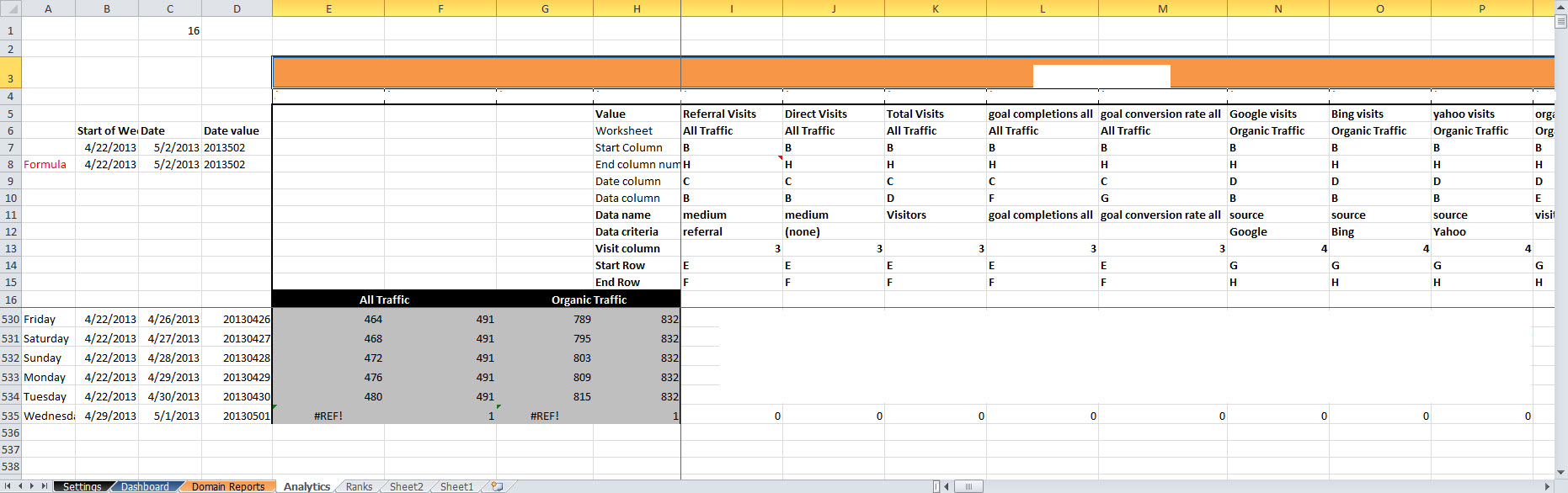
Two cells referenced give us the remainder of the file path instructions, Settings!B4 contains the file name format we’re using to end the analytics file names. 050113-analytics.xlsx. Then I6, not seen here is a cell reference we’re using to find the correct worksheet. If you want an idea of where this can take you, here’s an example of the formula and worksheet we use to track analytics data on all of our clients. We run analytics weekly but aggregate the data into one simple spreadsheet that makes it easy to graph and monitor each domain. It also organizes the data in a way that makes reporting dashboards easier to build and calculate our monthly reports.

That formula still makes my head spin, but it was created one piece at a time and tested one piece at a time to create the final product that it has become. When we first launched this new dashboard we incorporated historical analytics data that needed to be pulled into the spreadsheet, we pulled over 14 months of data for more than 20 domains in the first calculation of the sheet and it took less than 10 seconds to complete. When you consider the massive workload it needed to complete, 10 seconds is a miracle and obviously something I take some pride in. Here’s an example of the spreadsheet with all our typically hidden cells (for easier viewing) shown to reveal a small portion of the underpinnings behind this formula that is routed entirely in the use and abuse of the INDIRECT function to automate and accelerate data calculation and storage.